Discrete and Continuous Variables were defined in the article An Introduction to Frequency Distributions. We shall continue our discussion on frequency distributions in this article by moving on to Frequency Distributions of Discrete and Continuous Variables.
Frequency Distribution of a Discrete Variable
Since, a discrete variable can take some or discrete values within its range of variation, it will be natural to take a separate class for each distinct value of the discrete variable as shown in the following example relating to the daily number of car accidents during 30 days of a month.
3 4 4 5 5 3
4 3 5 7 6 4
4 3 4 5 5 5
5 5 3 5 6 4
5 4 4 6 5 6
Table No. 2: Showing frequency distribution for daily number of car accidents during a month.
| Number of car accidents | Frequency |
| 3 | 5 |
| 4 | 9 |
| 5 | 11 |
| 6 | 4 |
| 7 | 1 |
| Total | 30 |
Frequency Distribution of a Continuous Variable
For a continuous variable if we take a class for each distinct value of the variable, the number of classes will become unduly large, thus defeating the purpose of tabulation. In fact, since a continuous variable can assume an infinite number of values within its range of variation, the classification or sub-division of such data is necessarily artificial. Some guidelines that should be followed while dividing continuous data into classes are as follows:
- The classes should be mutually exclusive, i.e., non-overlapping. No two classes should contain the same interval of values of the variable.
- The classes should be exhaustive, i.e., they must cover the entire range of the data.
- The number of classes and the width of each class should neither be too small nor too large. In other words, there should be relatively fewer classes if the difference between the least value of the variable and its highest value is small and relatively more classes if the same difference is large. This difference between the least value of the variable and the greatest value of the variable is called the range of the variable or the data set.
- The classes should, preferably, be of equal width.
Let us consider the following example regarding daily maximum temperatures in

28 28 31 29 35 33 28 31 34 29
25 27 29 33 30 31 32 26 26 21
21 20 22 24 28 30 34 33 35 29
23 21 20 19 19 18 19 17 20 19
18 18 19 27 17 18 20 21 18 19
Minimum Value= 17
Maximum Value=35
Range=35-17=18
Number of classes=5 (say)


Table No. 3: Showing frequency distribution of temperature in a city for 50 days.
Class Intervals(Temperatures in  |
Frequency |
| 17-20 | 17 |
| 21-24 | 7 |
| 25-28 | 10 |
| 29-32 | 9 |
| 33-36 | 7 |
| Total | 50 |
Defining few terms
Class Interval: The whole range of variable values is classified in some groups in the form of intervals. Each interval is called a class interval.
Class Frequency: The number of observations in a class is termed as the frequency of the class or class frequency.
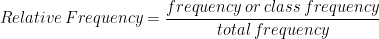
Relative Frequency: Relative frequency is defined as the proportion of observations corresponding to a particular value of the variable or a class of values of the variable. Relative frequency of a particular value of the variable or a class of values of the variable is obtained by dividing the frequency corresponding to that particular value or that particular class by the total number of observations in the data set, i.e., the total frequency.

Relative frequency of any value or any class lies between 0 and 1. We calculate relative frequency if we want an idea about the relative importance of the particular value or class in relation to the total frequency.
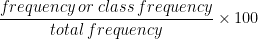
Percent Frequency: Sometimes Relative frequency is expressed in percent as


Class limits and Class boundaries:
Class limits are the two endpoints of a class interval which are used for the construction of a frequency distribution.The lowest value of the variable that can be included in a class interval is called the lower class limit of that class interval. The highest value of the variable that can be included in a class interval is called the upper class limit of that class interval. These are not the real limits or endpoints of a class interval. Hence, class limits are called apparent limits of a class.
Let us take for example, Table No. 3. The class intervals are 17-20, 21-24, 25-28, 29-32 and 33-36. Here, say for the class 17-20, the lower class limit is 17 and the upper class limit is 20. However, if there was an observation of 20.5, it would not be included in this class. An observation of 20.5 would be included in the class 21-24. Again if there was an observation of 16.5 it would be included in the class 17-20. Hence, effectively, the two actual endpoints of the class 17-20 are 16.5 and 20.5. These are actual or true limits of the class.
The two real endpoints of a class interval are called class boundaries. These are also called the real class limits. The basic rule is that class limits should have the same decimal place as the data set, but class boundaries should have one decimal place more. For example, let us say that we have the following data set on weight of a group of students (in Kg): 50.5, 50.8, 63.6, 48.4, 58.6, and 60.2. Here the class limits should have one decimal place and the class boundaries two decimal places. We obtain class boundaries from class limits by dividing the difference between the upper limit of a class and the lower limit of the next higher class into two equal parts. Say, we are considering the classes 17-20 and 21-24. 21-20=1. Again we have


Open-end classes: It may be so that some values in the data set are extremely small compared to the other values of the data set and similarly some values are extremely large in comparison. Then what we do is we do not use the lower limit of the first class and the upper limit of the last class. Such classes are called open end classes.
Class width: The length of the class is called the class width. It is also known as class size.


U.C.B. is Upper Class Boundary
L.C.B. is Lower Class Boundary
Class mark: The midpoint of a class interval is called class mark. It is the representative value of the entire class.


Frequency Density: It is the frequency per unit width of the class. It is given by:


Frequency densities are essential to compare two classes of unequal width. For classes equal class widths frequency densities are proportional to the class frequencies.
Relative Frequency Density: Relative frequency density of a class is relative frequency divided by the class width. It is given by:


Exercise
1. Construct a frequency distribution of the variable ‘word length’ from the following:
“Row row row your boat gentlt down the stream,
Merrily merrily, merrily merrily, life is but a dream.”
Calculate the relative frequencies and the percent frequencies.
2. The following data are based on the responses of 50 employees of a certain office on the distances (in Km) between their residence and workplace:
1.5 2.2 6.2 7.1 12.3 13.6 2.4 6.5 9.1 5.0
18.2 7.1 3.0 15.2 15.2 4.0 17.2 1.6 14.2 5.1
4.0 16.5 4.3 5.7 8.9 6.0 5.1 18.9 5.6 2.3
9.1 11.5 12.5 1.7 9.5 2.0 10.3 11.8 4.4 10.5
9.3 18.0 8.2 8.9 4.3 14.1 7.4 3.7 2.8 6.7
Construct the frequency distribution from this data.